How Hash Tables Work Under the Hood: The Secrets of Constant-Time O(1) Lookups
Basic Brain
Computer Science & Coding • November 09, 2026

How Hash Tables Work Under the Hood: The Secrets of Constant-Time O(1) Lookups
Imagine you are tasked with building a database to look up any citizen among a population of 1 billion people using their unique username.
If you store them in an unsorted list, finding a user requires checking every single record one by one. In computer science, this is an linear search. Scanning 1 billion items could take several seconds or minutes of pegging your CPU at 100%.
If you keep the list sorted alphabetically, you can perform a binary search (). For 1 billion items, that takes about 30 comparisons—vastly faster, but inserting a new user still forces you to shift hundreds of millions of elements in memory.
Enter the Hash Table (known as a dict in Python, an Object or Map in JavaScript, a HashMap in Java, and a map in Go and C++).
A hash table can find, insert, or delete any record in constant time: —whether you have 10 elements or 10 billion.
In this deep dive, we rip off the high-level abstraction to explore the mathematical machinery that makes hash tables the most critical data structure in computer engineering.
1. The Core Architecture: Arrays + Math
Underneath all the syntactic sugar of user["elisha"] = data, computers only truly understand one primitive, contiguous data structure: an array in memory.
An array gives you instant access if and only if you know the numerical memory index:
const users = ["Alice", "Bob", "Charlie"];
console.log(users[0]); // Instant O(1) access
The fundamental problem of computing is that humans don't look up data by integer indices like users[42918]; we look up data by meaningful strings like "user_id_99" or "session_token".
A Hash Table solves this by inserting a mathematical translation bridge:
[ Key: "username" ] ───> [ Hash Function h(k) ] ───> [ Modulo Array Size ] ───> Index [ 3 ]
- You feed your key (e.g.,
"basicbrain") into a Hash Function. - The hash function converts the characters into a massive integer (e.g.,
2,849,102,841). - You take the modulo of that integer with the size of your storage array (
2,849,102,841 % 16 = 9). - The computer jumps directly to index
9in RAM and retrieves the value in a single CPU memory cycle.

2. What Makes a Good Hash Function?
A hash function is not an encryption algorithm like AES or RSA; it is designed for raw throughput and uniform distribution. A high-performance hash function must satisfy four rules:
- Deterministic: Passing
"apple"must always produce the exact same integer every single time. - Fast (): Computing the hash must take minimal CPU cycles (typically using bitwise XOR, shifts, and 64-bit integer multiplication).
- Uniform Distribution: Keys should scatter evenly across all available buckets rather than piling up in one spot.
- The Avalanche Effect: Changing a single bit in the input (e.g.
"cat"vs"car") should drastically change the resulting hash value so nearby strings don't cluster.
Popular Production Hash Algorithms
- FNV-1a (Fowler–Noll–Vo): Ultra-fast, simple, non-cryptographic hash algorithm based on prime multiplication and XOR folding.
- MurmurHash3 & CityHash: High-performance algorithms developed by Google and Austin Appleby used in distributed databases (Cassandra, Hadoop).
- SipHash: Cryptographically hardened against HashDoS attacks, where malicious actors intentionally craft colliding keys to slow web servers down from to . Python and Rust use SipHash by default.
3. The Inevitable Problem: Collisions
There are infinitely many possible string keys, but your computer has a finite number of array slots.
By the Pigeonhole Principle, if you have 100 slots in an array and you insert 101 keys, at least two keys must map to the exact same index. This is called a Hash Collision.
Even with far fewer items, the Birthday Paradox proves that in an array of 365 slots, having just 23 keys creates a 50% probability of a collision!
Engineers have developed two primary strategies to handle collisions.
4. Collision Resolution 1: Separate Chaining
In Separate Chaining, each index of the array does not hold a single value; it holds a pointer to a Linked List (or dynamic bucket array).
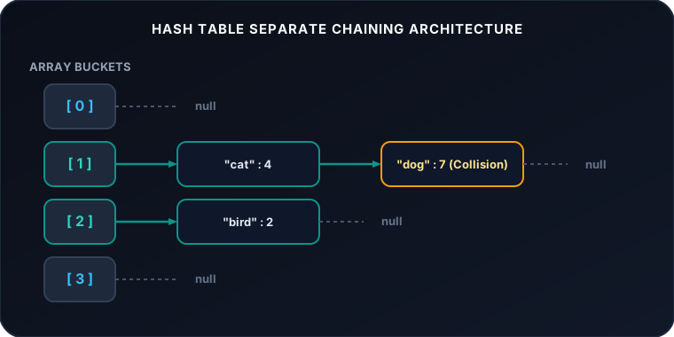
- Insertion: Hash the key. Jump to the bucket. Append the new key-value pair to the linked list: .
- Lookup: Hash the key. Jump to the bucket. Walk down the linked list until you find the exact key: where is the length of the list.
Java 8 Optimization: If a bucket's linked list grows beyond 8 elements, Java automatically transforms that linked list into a Red-Black Balanced Binary Search Tree. This guarantees that even under catastrophic collision conditions, lookups never degrade worse than .
5. Collision Resolution 2: Open Addressing
In Open Addressing, there are no linked lists. Every key-value pair is stored directly inside the main array. If slot is already occupied, the algorithm searches ("probes") for another empty slot:
- Linear Probing: If slot is full, check sequentially.
- Drawback: Causes Primary Clustering—long clusters of occupied slots merge together, severely degrading performance.
- Quadratic Probing: Check slots with quadratic step sizes: to break up clusters.
- Double Hashing: Use a second hash function to calculate a custom step size for each key:
- Robin Hood Hashing: During insertion, if a new element has traveled farther from its home bucket than the current occupant, the new element "steals" the slot and kicks the existing occupant further down. This equalizes probe lengths across the entire table.

6. The Load Factor & Dynamic Resizing
As you insert more items into a hash table, collisions multiply and lookup speeds degrade. How does a hash table maintain its constant-time speed?
It tracks the Load Factor ():
Where:
- = The total number of items currently stored.
- = The total number of allocated buckets (array capacity).
When reaches or , the hash table automatically executes a Dynamic Rehash:
- It allocates a brand-new internal array with double the capacity ().
- It iterates through every single key-value pair in the old array, recalculates its new index:
- It moves all elements into the new array and discards the old array.
Although resizing takes time, it happens so infrequently that the cost is distributed across thousands of insertions. In computer science, this is known as Amortized time.
7. Building a Working Hash Table in TypeScript
Here is a clean, dependency-free implementation demonstrating FNV-1a hashing, separate chaining, and automatic lookups:
class SimpleHashTable<V> {
  private buckets: Array<Array<[string, V]>>;
  private size: number = 0;
  private capacity: number;
  private readonly loadFactorThreshold = 0.75;

  constructor(initialCapacity = 16) {
    this.capacity = initialCapacity;
    this.buckets = new Array(this.capacity).fill(null).map(() => []);
  }

  // Fast 32-bit FNV-1a Hash Algorithm
  private hash(key: string): number {
    let hash = 2166136261;
    for (let i = 0; i < key.length; i++) {
      hash ^= key.charCodeAt(i);
      hash = Math.imul(hash, 16777619);
    }
    return (hash >>> 0) % this.capacity;
  }

  // O(1) Amortized Insert
  public set(key: string, value: V): void {
    const index = this.hash(key);
    const bucket = this.buckets[index];

    // Update if key already exists
    for (let i = 0; i < bucket.length; i++) {
      if (bucket[i][0] === key) {
        bucket[i][1] = value;
        return;
      }
    }

    // Insert new entry
    bucket.push([key, value]);
    this.size++;

    // Check load factor and resize if needed
    if (this.size / this.capacity >= this.loadFactorThreshold) {
      this.resize(this.capacity * 2);
    }
  }

  // O(1) Average Lookup
  public get(key: string): V | undefined {
    const index = this.hash(key);
    const bucket = this.buckets[index];

    for (const [k, v] of bucket) {
      if (k === key) return v;
    }
    return undefined;
  }

  // Dynamic Rehashing to double capacity
  private resize(newCapacity: number): void {
    const oldBuckets = this.buckets;
    this.capacity = newCapacity;
    this.buckets = new Array(this.capacity).fill(null).map(() => []);
    this.size = 0;

    for (const bucket of oldBuckets) {
      for (const [k, v] of bucket) {
        this.set(k, v);
      }
    }
  }
}

// Usage Demo
const map = new SimpleHashTable<number>();
map.set("transistors", 1947);
map.set("resistors", 1827);

console.log(map.get("transistors")); // Output: 1947
8. Data Structure Showdown
| Data Structure | Access | Search (Lookup) | Insertion | Deletion | Space Complexity |
|---|---|---|---|---|---|
| Array (Unsorted) | |||||
| Array (Sorted) | |||||
| Binary Search Tree (AVL/Red-Black) | |||||
| Hash Table (Average Case) | |||||
| Hash Table (Worst Case - Collisions) |

9. Watch the Video Breakdown
Seeing memory allocation and collision resolution animated visually makes the concept intuitive. Watch this comprehensive algorithmic breakdown:
More Computer Science & Engineering
For more breakdowns of algorithms, electronics, hardware architecture, and deep technical explainers, follow along on:
- 🎥 Basic Brain on YouTube (@basicbraincut) — Visual explorations of how real-world machines, semiconductors, and software architectures operate.
10. Key Takeaways
- Arrays provide the speed: Hash tables leverage the physical memory addressing of RAM to achieve constant-time access.
- Hash functions translate strings to indices: Using bitwise mathematics and modulo operations ().
- Collisions are guaranteed: By the Pigeonhole Principle. They are solved via Separate Chaining (linked lists/trees) or Open Addressing (probing).
- Dynamic resizing keeps it fast: When the load factor reaches , doubling the table and redistributing elements keeps search buckets shallow.
Written & curated for the Basic Brain technical library. What algorithmic concept or data structure should we break down next? Leave your thoughts in the comments below!